Launch this notebook on on mybinder.org:

---

Transport Map from density

The objective of this example is to show how a transport map can be build in MParT when the the unnormalized probability density function of the target density is known.

Problem description

We consider \(T(\mathbf{z};\mathbf{w})\) a monotone triangular transport map parameterized by \(\mathbf{w}\) (e.g., polynomial coefficients). This map which is invertible and has an invertible Jacobian for any parameter \(\mathbf{w}\), transports samples \(\mathbf{z}^i\) from the reference density \(\eta\) to samples \(T(\mathbf{z}^i;\mathbf{w})\) from the map induced density \(\tilde{\pi}_\mathbf{w}(\mathbf{z})\) defined as:

\[\tilde{\pi}_\mathbf{w}(\mathbf{z}) = \eta(T^{-1}(\mathbf{z};\mathbf{w}))|\text{det } T^{-1}(\mathbf{z};\mathbf{w})|,\]

where \(\text{det } T^{-1}\) is the determinant of the inverse map Jacobian at the point \(\mathbf{z}\). We refer to \(\tilde{\pi}_{\mathbf{w}}(\mathbf{x})\) as the map-induced density or pushforward distribution and will commonly interchange notation for densities and measures to use the notation \(\tilde{\pi} = T_{\sharp} \eta\).

The objective of this example is, knowing some unnormalized target density \(\bar{\pi}\), find the map \(T\) that transport samples drawn from \(\eta\) to samples drawn from the target \(\pi\).

Imports

First, import MParT and other packages used in this notebook. Note that it is possible to specify the number of threads used by MParT by setting the KOKKOS_NUM_THREADS environment variable before importing MParT.

import numpy as np
from scipy.optimize import minimize
import matplotlib.pyplot as plt
from scipy.stats import multivariate_normal

import os
os.environ['KOKKOS_NUM_THREADS'] = '8'

import mpart as mt
print('Kokkos is using', mt.Concurrency(), 'threads')
plt.rcParams['figure.dpi'] = 110

Kokkos::OpenMP::initialize WARNING: You are likely oversubscribing your CPU cores.
  process threads available :   4,  requested thread :   8

Kokkos::OpenMP::initialize WARNING: You are likely oversubscribing your CPU cores.
                                    Detected: 4 cores per node.
                                    Detected: 1 MPI_ranks per node.
                                    Requested: 8 threads per process.

Kokkos is using 8 threads

Target density and exact map

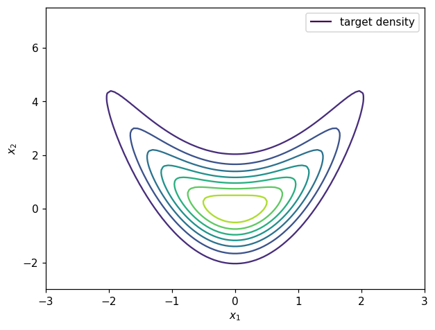
In this example we use a 2D target density known as the banana density where the unnormalized probability density, samples and the exact transport map are known.

The banana density is defined as:

\[\pi(x_1,x_2) \propto N_1(x_1)\times N_1(x_2-x_1^2)\]

where \(N_1\) is the 1D standard normal density.

The exact transport map that transport the 2D standard normal density to \(\pi\) is known as:

\[\begin{split} {T}^\text{true}(z_1,z_2)= \begin{bmatrix} z_1\\ z_2 + z_1^2 \end{bmatrix}\end{split}\]

Contours of the target density can be visualized as:

# Unnomalized target density required for objective
def target_logpdf(x):
  rv1 = multivariate_normal(np.zeros(1),np.eye(1))
  rv2 = multivariate_normal(np.zeros(1),np.eye(1))
  logpdf1 = rv1.logpdf(x[0])
  logpdf2 = rv2.logpdf(x[1]-x[0]**2)
  logpdf = logpdf1 + logpdf2
  return logpdf

# Grid for plotting
ngrid=100
x1_t = np.linspace(-3,3,ngrid)
x2_t = np.linspace(-3,7.5,ngrid)
xx1,xx2 = np.meshgrid(x1_t,x2_t)

xx = np.vstack((xx1.reshape(1,-1),xx2.reshape(1,-1)))

# Target contours
target_pdf_at_grid = np.exp(target_logpdf(xx))

fig, ax = plt.subplots()
CS1 = ax.contour(xx1, xx2, target_pdf_at_grid.reshape(ngrid,ngrid))
ax.set_xlabel(r'$x_1$')
ax.set_ylabel(r'$x_2$')
h1,_ = CS1.legend_elements()
legend1 = ax.legend([h1[0]], ['target density'])
plt.show()

Map training

Defining objective function and its gradient

Knowing the closed form of the unnormalized target density \(\bar{\pi}\), the objective is to find a map-induced density \(\tilde{\pi}_{\mathbf{w}}(\mathbf{z})\) that is a good approximation of the target \(\pi\).

In order to characterize this posterior density, one method is to build a monotone triangular transport map \(T\) such that the KL divergence \(D_{KL}(\eta || T^\sharp \pi)\) is minmized. If \(T\) is map parameterized by \(\mathbf{w}\), the objective function derived from the discrete KL divergence reads:

\[J(\mathbf{w}) = - \frac{1}{N}\sum_{i=1}^N \left( \log\pi\left(T(\mathbf{z}^i;\mathbf{w})\right) + \log \text{det }\nabla_\mathbf{z} T(\mathbf{z}^i;\mathbf{w})\right), \,\,\, \mathbf{z}^i \sim \mathcal{N}(\mathbf{0},\mathbf{I}_d),\]

where \(T\) is the transport map pushing forward the standard normal \(\mathcal{N}(\mathbf{0},\mathbf{I}_d)\) to the target density \(\pi(\mathbf{z})\). The gradient of this objective function reads

\[\nabla_\mathbf{w} J(\mathbf{w}) = - \frac{1}{N}\sum_{i=1}^N \left( \nabla_\mathbf{w} T(\mathbf{z}^i;\mathbf{w}).\nabla_\mathbf{x}\log\pi\left(T(\mathbf{z}^i;\mathbf{w})\right) + \nabla_{\mathbf{w}}\log \text{det }\nabla_\mathbf{z} T(\mathbf{z}^i;\mathbf{w})\right), \,\,\, \mathbf{z}^i \sim \mathcal{N}(\mathbf{0},\mathbf{I}_d).\]

The objective function and gradient can be defined using MParT as:

# KL divergence objective
def obj(coeffs, transport_map, x):
    num_points = x.shape[1]
    transport_map.SetCoeffs(coeffs)
    map_of_x = transport_map.Evaluate(x)
    logpdf= target_logpdf(map_of_x)
    log_det = transport_map.LogDeterminant(x)
    return -np.sum(logpdf + log_det)/num_points

# Gradient of unnomalized target density required for gradient objective
def target_grad_logpdf(x):
  grad1 = -x[0,:] + (2*x[0,:]*(x[1,:]-x[0,:]**2))
  grad2 = (x[0,:]**2-x[1,:])
  return np.vstack((grad1,grad2))

# Gradient of KL divergence objective
def grad_obj(coeffs, transport_map, x):
    num_points = x.shape[1]
    transport_map.SetCoeffs(coeffs)
    map_of_x = transport_map.Evaluate(x)
    sens_vecs = target_grad_logpdf(map_of_x)
    grad_logpdf = transport_map.CoeffGrad(x, sens_vecs)
    grad_log_det = transport_map.LogDeterminantCoeffGrad(x)
    return -np.sum(grad_logpdf + grad_log_det, 1)/num_points

Map parameterization

For the parameterization of \(T\) we use a total order multivariate expansion of hermite functions. Knowing \(T^\text{true}\), any parameterization with total order greater than one will include the true solution of the map finding problem.

# Set-up first component and initialize map coefficients
map_options = mt.MapOptions()

total_order = 2

# Create dimension 2 triangular map
transport_map = mt.CreateTriangular(2,2,total_order,map_options)

Approximation before optimization

Coefficients of triangular map are set to 0 upon creation.

# Make reference samples for training
num_points = 10000
z = np.random.randn(2,num_points)

# Make reference samples for testing
test_z = np.random.randn(2,5000)

# Pushed samples
x = transport_map.Evaluate(test_z)

# Before optimization plot
plt.figure()
plt.contour(xx1, xx2, target_pdf_at_grid.reshape(ngrid,ngrid))
plt.scatter(x[0],x[1], facecolor='blue', alpha=0.1, label='Pushed samples')
plt.legend()
plt.show()

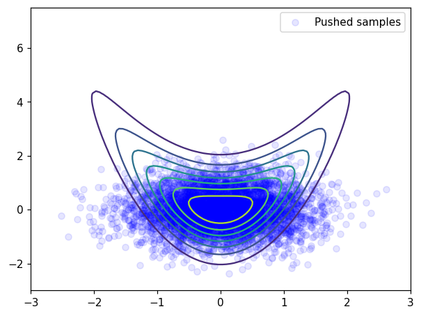
At initialization, samples are “far” from being distributed according to the banana distribution.

Initial objective and coefficients:

# Print initial coeffs and objective
print('==================')
print('Starting coeffs')
print(transport_map.CoeffMap())
print('Initial objective value: {:.2E}'.format(obj(transport_map.CoeffMap(), transport_map, test_z)))
print('==================')

==================
Starting coeffs
[0. 0. 0. 0. 0. 0. 0. 0. 0.]
Initial objective value: 3.40E+00
==================

Minimization

print('==================')
options={'gtol': 1e-4, 'disp': True}
res = minimize(obj, transport_map.CoeffMap(), args=(transport_map, z), jac=grad_obj, method='BFGS', options=options)

# Print final coeffs and objective
print('Final coeffs:')
print(transport_map.CoeffMap())
print('Final objective value: {:.2E}'.format(obj(transport_map.CoeffMap(), transport_map, test_z)))
print('==================')

==================

Optimization terminated successfully.
         Current function value: 2.848868
         Iterations: 17
         Function evaluations: 19
         Gradient evaluations: 19
Final coeffs:
[ 1.64386417e-02  8.40185180e-01  1.11002314e-02  9.88287812e-01
  8.46815229e-01 -7.30824747e-03  7.15717444e-02 -1.61399131e-03
  2.21101864e+00]
Final objective value: 2.83E+00
==================

Approximation after optimization

Pushed samples

# Pushed samples
x = transport_map.Evaluate(test_z)

# After optimization plot
plt.figure()
plt.contour(xx1, xx2, target_pdf_at_grid.reshape(ngrid,ngrid))
plt.scatter(x[0],x[1], facecolor='blue', alpha=0.1, label='Pushed samples')
plt.legend()
plt.show()

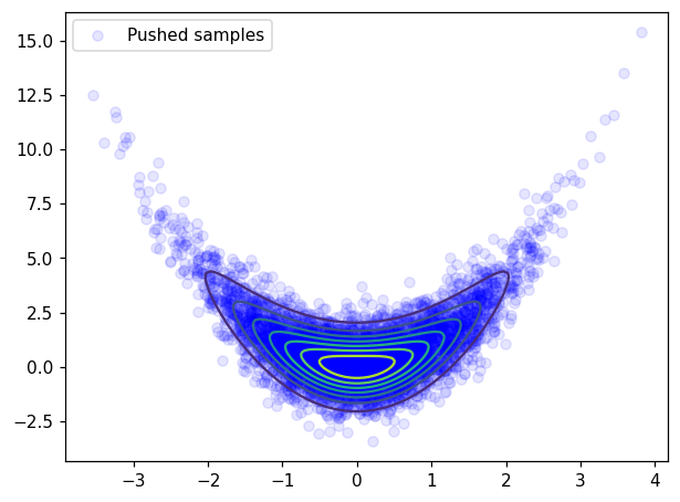
After optimization, pushed samples \(T(z^i)\), \(z^i \sim \mathcal{N}(0,I)\) are approximately distributed according to the target \(\pi\)

Variance diagnostic

A commonly used accuracy check when facing computation maps from density is the so-called variance diagnostic defined as:

\[\epsilon_\sigma = \frac{1}{2} \mathbb{V}\text{ar}_\rho \left[ \log \frac{\rho}{T^\sharp \bar{\pi}} \right]\]

This diagnostic is asymptotically equivalent to the minimized KL divergence \(D_{KL}(\eta || T^\sharp \pi)\) and should converge to zero when the computed map converge to the true map.

The variance diagnostic can be computed as follow:

def variance_diagnostic(tri_map,ref,target_logpdf,x):
  ref_logpdf = ref.logpdf(x.T)
  y = tri_map.Evaluate(x)
  pullback_logpdf = target_logpdf(y) + tri_map.LogDeterminant(x)
  diff = ref_logpdf - pullback_logpdf
  expect = np.mean(diff)
  var = 0.5*np.mean((diff-expect)**2)
  return var

# Reference distribution
ref_distribution = multivariate_normal(np.zeros(2),np.eye(2));

# Compute variance diagnostic
var_diag = variance_diagnostic(transport_map,ref_distribution,target_logpdf,test_z)

# Print variance diagnostic
print('==================')
print('Variance diagnostic: {:.2E}'.format(var_diag))
print('==================')

==================
Variance diagnostic: 3.34E-04
==================

Pushforward density

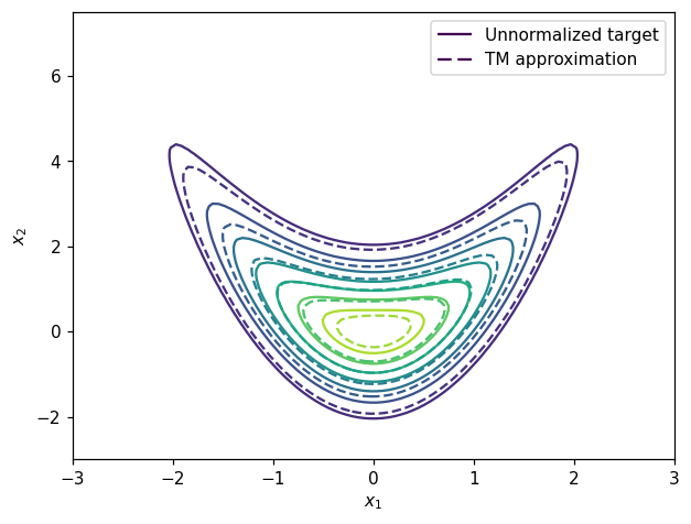
We can also plot the contour of the unnormalized density \(\bar{\pi}\) and the pushforward approximation \(T_\sharp \eta\):

# Pushforward definition
def push_forward_pdf(tri_map,ref,x):
  xinv = tri_map.Inverse(x,x)
  log_det_grad_x_inverse = - tri_map.LogDeterminant(xinv)
  log_pdf = ref.logpdf(xinv.T)+log_det_grad_x_inverse
  return np.exp(log_pdf)

map_approx_grid = push_forward_pdf(transport_map,ref_distribution,xx)

fig, ax = plt.subplots()
CS1 = ax.contour(xx1, xx2, target_pdf_at_grid.reshape(ngrid,ngrid))
CS2 = ax.contour(xx1, xx2, map_approx_grid.reshape(ngrid,ngrid),linestyles='--')
ax.set_xlabel(r'$x_1$')
ax.set_ylabel(r'$x_2$')
h1,_ = CS1.legend_elements()
h2,_ = CS2.legend_elements()
legend1 = ax.legend([h1[0], h2[0]], ['Unnormalized target', 'TM approximation'])
plt.show()