Launch this notebook on on mybinder.org:
Characterization of Bayesian posterior density#
The objective of this example is to demonstrate how transport maps can be used to represent posterior distribution of Bayesian inference problems.
Imports#
First, import MParT and other packages used in this notebook. Note that it is possible to specify the number of threads used by MParT by setting the KOKKOS_NUM_THREADS environment variable before importing MParT.
[1]:
import numpy as np
import scipy
from scipy.optimize import minimize
import matplotlib.pyplot as plt
from scipy.stats import multivariate_normal

import os
os.environ['KOKKOS_NUM_THREADS'] = '8'

import mpart as mt
print('Kokkos is using', mt.Concurrency(), 'threads')
plt.rcParams['figure.dpi'] = 110
Kokkos::OpenMP::initialize WARNING: You are likely oversubscribing your CPU cores.
  process threads available :   4,  requested thread :   8
Kokkos::OpenMP::initialize WARNING: You are likely oversubscribing your CPU cores.
                                    Detected: 4 cores per node.
                                    Detected: 1 MPI_ranks per node.
                                    Requested: 8 threads per process.
Kokkos is using 8 threads
Problem formulation#
Bayesian inference#
A way construct a transport map is from an unnormalized density. One situation where we know the probality density function up to a normalization constant is when modeling inverse problems with Bayesian inference.
For an inverse problem, the objective is to characterize the value of some parameters \(\boldsymbol{\theta}\) of a given system, knowing some the value of some noisy observations \(\mathbf{y}\).
With Bayesian inference, the characterization of parameters \(\boldsymbol{\theta}\) is done via a posterior density \(\pi(\boldsymbol{\theta}|\mathbf{y})\). This density characterizes the distribution of the parameters knowing the value of the observations.
Using Bayes’ rule, the posterior can decomposed into the product of two probability densities:
The prior density \(\pi(\boldsymbol{\theta})\) which is used to enforce any a priori knowledge about the parameters.
The likelihood function \(\pi(\mathbf{y}|\boldsymbol{\theta})\). This quantity can be seen as a function of \(\boldsymbol{\theta}\) and gives the likelihood that the considered system produced the observation \(\mathbf{y}\) for a fixed value of \(\boldsymbol{\theta}\). When the model that describes the system is known in closed form, the likelihood function is also knwon in closed form.
Hence, the posterior density reads:
where \(c = \int \pi(\mathbf{y}|\boldsymbol{\theta}) \pi(\boldsymbol{\theta}) d\theta\) is an normalizing constant that ensures that the product of the two quantities is a proper density. Typically, the integral in this definition cannot be evaluated and \(c\) is assumed to be unknown.
The objective of this examples is, from the knowledge of \(\pi(\mathbf{y}|\boldsymbol{\theta})\pi(\boldsymbol{\theta})\) build a transport map that transports samples from the reference \(\eta\) to samples from posterior \(\pi(\boldsymbol{\theta}|\mathbf{y})\).
Application with the Biochemical Oxygen Demand (BOD) model from [Sullivan et al., 2010]#
Definition#
To illustrate the process describe above, we consider the BOD inverse problem described in [Marzouk et al., 2016]. The goal is to estimate \(2\) coefficients in a time-dependent model of oxygen demand, which is used as an indication of biological activity in a water sample.
The time dependent forward model is defined as
where
The objective is to characterize the posterior density of parameters \(\boldsymbol{\theta}=(\theta_1,\theta_2)\) knowing observation of the system at time \(t=\left\{1,2,3,4,5 \right\}\) i.e. \(\mathbf{y} = (y_1,y_2,y_3,y_4,y_5) = (\mathcal{B}(1),\mathcal{B}(2),\mathcal{B}(3),\mathcal{B}(4),\mathcal{B}(5))\).
Definition of the forward model and gradient with respect to \(\mathbf{\theta}\):
[2]:
def forward_model(p1,p2,t):
  A = 0.4+0.4*(1+scipy.special.erf(p1/np.sqrt(2)))
  B = 0.01+0.15*(1+scipy.special.erf(p2/np.sqrt(2)))
  out = A*(1-np.exp(-B*t))
  return out

def grad_x_forward_model(p1,p2,t):
  A = 0.4+0.4*(1+scipy.special.erf(p1/np.sqrt(2)))
  B = 0.01+0.15*(1+scipy.special.erf(p2/np.sqrt(2)))
  dAdx1 = 0.31954*np.exp(-0.5*p1**2)
  dBdx2 = 0.119683*np.exp(-0.5*p2**2)
  dOutdx1 = dAdx1*(1-np.exp(-B*t))
  dOutdx2 = t*A*dBdx2*np.exp(-t*B)
  return np.vstack((dOutdx1,dOutdx2))
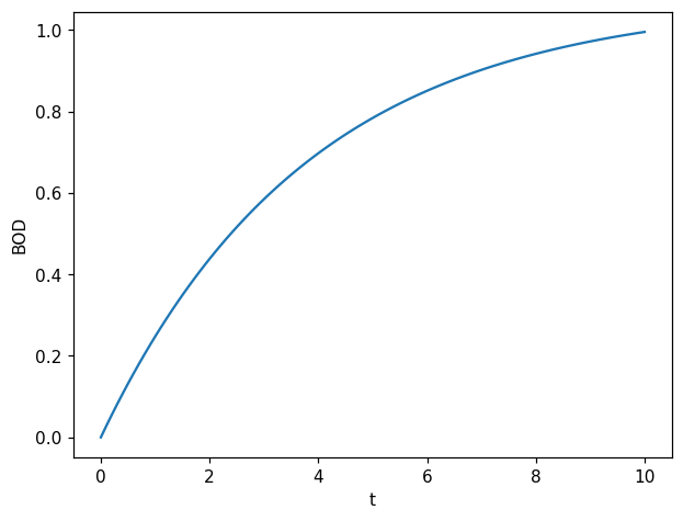
One simulation of the forward model:
[3]:
t = np.linspace(0,10, 100)
fig, ax = plt.subplots(1,1)
ax.plot(t, forward_model(1, 1, t));
ax.set_xlabel("t")
ax.set_ylabel("BOD");
For this problem, as noise \(\mathcal{E}\) is Gaussian and additive, the likelihood function \(\pi(\mathbf{y}|\boldsymbol{\theta})\), can be decomposed for each time step as:
where
Likelihood function and its gradient with respect to parameters:
[4]:
def log_likelihood(std_noise,t,yobs,p1,p2):
  y = forward_model(p1,p2,t)
  log_lkl = -np.log(np.sqrt(2*np.pi)*std_noise)-0.5*((y-yobs)/std_noise)**2
  return log_lkl

def grad_x_log_likelihood(std_noise,t,yobs,p1,p2):
  y = forward_model(p1,p2,t)
  dydx = grad_x_forward_model(p1,p2,t)
  grad_x_lkl = (-1/std_noise**2)*(y - yobs)*dydx
  return grad_x_lkl
We can then define the unnormalized posterior and its gradient with respect to parameters:
[5]:
def log_posterior(std_noise,std_prior1,std_prior2,list_t,list_yobs,p1,p2):
  log_prior1 = -np.log(np.sqrt(2*np.pi)*std_prior1)-0.5*(p1/std_prior1)**2
  log_prior2 = -np.log(np.sqrt(2*np.pi)*std_prior2)-0.5*(p2/std_prior2)**2
  log_posterior = log_prior1+log_prior2
  for k,t in enumerate(list_t):
    log_posterior += log_likelihood(std_noise,t,list_yobs[k],p1,p2)
  return log_posterior

def grad_x_log_posterior(std_noise,std_prior1,std_prior2,list_t,list_yobs,p1,p2):
  grad_x1_prior = -(1/std_prior1**2)*(p1)
  grad_x2_prior = -(1/std_prior2**2)*(p2)
  grad_x_prior = np.vstack((grad_x1_prior,grad_x2_prior))
  grad_x_log_posterior = grad_x_prior
  for k,t in enumerate(list_t):
    grad_x_log_posterior += grad_x_log_likelihood(std_noise,t,list_yobs[k],p1,p2)
  return grad_x_log_posterior
Observations#
We consider the following realization of observation \(\mathbf{y}\):
[6]:
list_t = np.array([1,2,3,4,5])
list_yobs = np.array([0.18,0.32,0.42,0.49,0.54])

std_noise = np.sqrt(1e-3)
std_prior1 = 1
std_prior2 = 1
Visualization of the unnormalized posterior density#
[7]:
Ngrid = 100
x = np.linspace(-0.5, 1.25, Ngrid)
y = np.linspace(-0.5, 2.5, Ngrid)
X, Y = np.meshgrid(x, y)

Z = log_posterior(std_noise,std_prior1,std_prior2,list_t,list_yobs,X.flatten(),Y.flatten())
Z = np.exp(Z.reshape(Ngrid,Ngrid))


fig, ax = plt.subplots()
CS = ax.contour(X, Y, Z)
ax.set_xlabel(r'$\theta_1$')
ax.set_ylabel(r'$\theta_2$')
plt.show()
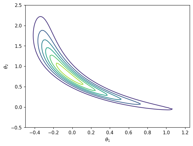
Target density for the map from density is non-Gaussian which mean that a non linear map will be required to achieve good approximation.
Map computation#
After the definition of the log-posterior and gradient, the construction of the desired map \(T\) to characterize the posterior density result in a “classic” map from unnomarlized computation.
Definition of the objective function:#
Knowing the closed form of unnormalized posterior \(\bar{\pi}(\boldsymbol{\theta} |\mathbf{y})= \pi(\mathbf{y}|\boldsymbol{\theta})\pi(\boldsymbol{\theta})\), the objective is to find a map-induced density \(\tilde{\pi}_{\mathbf{w}}(\mathbf{x})\) that is a good approximation to the posterior \(\pi(\boldsymbol{\theta} |\mathbf{y})\).
In order to characterize this posterior density, one method is to build a transport map.
For the map from unnormalized density estimation, the objective function on parameter \(\mathbf{w}\) reads:
where \(T\) is the transport map pushing forward the standard normal \(\mathcal{N}(\mathbf{0},\mathbf{I}_d)\) to the target density \(\pi(\mathbf{x})\), which will be the the posterior density. The gradient of this objective function reads:
[8]:
def grad_x_log_target(x):
  out = grad_x_log_posterior(std_noise,std_prior1,std_prior2,list_t,list_yobs,x[0,:],x[1,:])
  return out

def log_target(x):
  out = log_posterior(std_noise,std_prior1,std_prior2,list_t,list_yobs,x[0,:],x[1,:])
  return out

def obj(coeffs, tri_map,x):
    num_points = x.shape[1]
    tri_map.SetCoeffs(coeffs)
    map_of_x = tri_map.Evaluate(x)
    rho_of_map_of_x = log_target(map_of_x)
    log_det = tri_map.LogDeterminant(x)
    return -np.sum(rho_of_map_of_x + log_det)/num_points

def grad_obj(coeffs, tri_map, x):
    num_points = x.shape[1]
    tri_map.SetCoeffs(coeffs)
    map_of_x = tri_map.Evaluate(x)
    sensi = grad_x_log_target(map_of_x)
    grad_rho_of_map_of_x = tri_map.CoeffGrad(x, sensi)
    grad_log_det = tri_map.LogDeterminantCoeffGrad(x)
    return -np.sum(grad_rho_of_map_of_x + grad_log_det, 1)/num_points
[9]:
#Draw reference samples to define objective
N=10000
z = np.random.randn(2,N)
Map parametrization#
We use the MParT function CreateTriangular to directly create a transport map object of dimension with given total order parameterization.
[10]:
# Create transport map
opts = mt.MapOptions()
total_order = 3
tri_map = mt.CreateTriangular(2,2,total_order,opts)
Optimization#
[11]:
options={'gtol': 1e-2, 'disp': True}
res = scipy.optimize.minimize(obj, tri_map.CoeffMap(), args=(tri_map, z), jac=grad_obj, method='BFGS', options=options)
Optimization terminated successfully.
         Current function value: -6.250160
         Iterations: 29
         Function evaluations: 36
         Gradient evaluations: 36
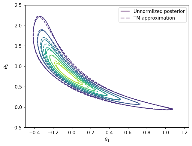
Accuracy checks#
Comparing density contours#
Comparison between contours of the posterior \(\pi(\boldsymbol{\theta}|\mathbf{y})\) and conoturs of pushforward density \(T_\sharp \eta\).
[12]:
# Pushforward distribution
def push_forward_pdf(tri_map,ref,x):
  xinv = tri_map.Inverse(x,x)
  log_det_grad_x_inverse = - tri_map.LogDeterminant(xinv)
  log_pdf = ref.logpdf(xinv.T)+log_det_grad_x_inverse
  return np.exp(log_pdf)
[13]:
# Reference distribution
ref = multivariate_normal(np.zeros(2),np.eye(2))

xx_eval = np.vstack((X.flatten(),Y.flatten()))
Z2 = push_forward_pdf(tri_map,ref,xx_eval)
Z2 = Z2.reshape(Ngrid,Ngrid)

fig, ax = plt.subplots()
CS1 = ax.contour(X, Y, Z)
CS2 = ax.contour(X, Y, Z2,linestyles='dashed')
ax.set_xlabel(r'$\theta_1$')
ax.set_ylabel(r'$\theta_2$')
h1,_ = CS1.legend_elements()
h2,_ = CS2.legend_elements()
ax.legend([h1[0], h2[0]], ['Unnormilzed posterior', 'TM approximation'])
plt.show()
Variance diagnostic#
A commonly used accuracy check when facing computation maps from density is the so-called variance diagnostic defined as:
This diagnostic is asymptotically equivalent to the minimized KL divergence \(D_{KL}(\eta || T^\sharp \pi)\) and should converge to zero when the computed map converge to the theoritical true map.
[14]:
def variance_diagnostic(tri_map,ref,target_logpdf,x):
  ref_logpdf = ref.logpdf(x.T)
  y = tri_map.Evaluate(x)
  pullback_logpdf = target_logpdf(y) + tri_map.LogDeterminant(x)
  diff = ref_logpdf - pullback_logpdf
  expect = np.mean(diff)
  var = 0.5*np.mean((diff-expect)**2)
  return var
[15]:
# Reference distribution
ref_distribution = multivariate_normal(np.zeros(2),np.eye(2));

test_z = np.random.randn(2,10000)
# Compute variance diagnostic
var_diag = variance_diagnostic(tri_map,ref,log_target,test_z)

# Print final coeffs and objective
print('==================')
print('Variance diagnostic: {:.2E}'.format(var_diag))
print('==================')
==================
Variance diagnostic: 4.95E-02
==================
Drawing samples from approximate posterior#
Once the transport map from reference to unnormalized posterior is estimated it can be used to sample from the posterior to characterize the Bayesian inference solution.
[16]:
Znew = np.random.randn(2,5000)
colors = np.arctan2(Znew[1,:],Znew[0,:])

Xpost = tri_map.Evaluate(Znew)

fig,axs = plt.subplots(ncols=2,figsize=(12,5))
axs[0].scatter(Xpost[0,:],Xpost[1,:], c=colors, alpha=0.2)
axs[0].set_aspect('equal', 'box')
axs[0].set_xlabel(r'$\theta_1$')
axs[0].set_ylabel(r'$\theta_2$')
axs[0].set_title('Approximate Posterior Samples')

axs[1].scatter(Znew[0,:],Znew[1,:], c=colors, alpha=0.2)
axs[1].set_aspect('equal', 'box')
axs[1].set_xlabel(r'$z_1$')
axs[1].set_ylabel(r'$z_2$')
axs[1].set_title('Reference Samples')


plt.show()
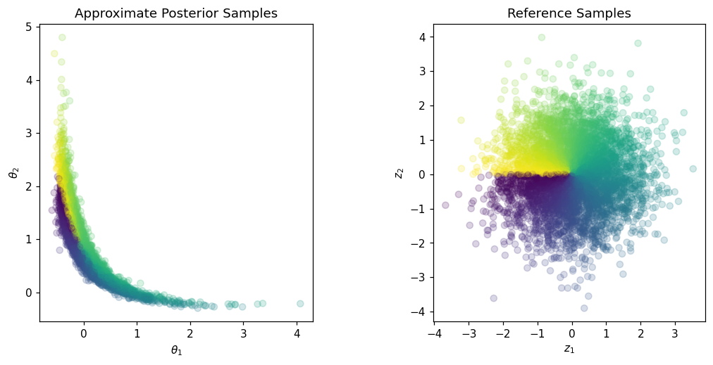
Samples can then be used to compute quantity of interest with respect to parameters \(\boldsymbol{\theta}\). For example the sample mean:
[17]:
X_mean = np.mean(Xpost,1)
print('Mean a posteriori: '+str(X_mean))
Mean a posteriori: [0.03338503 0.92169768]
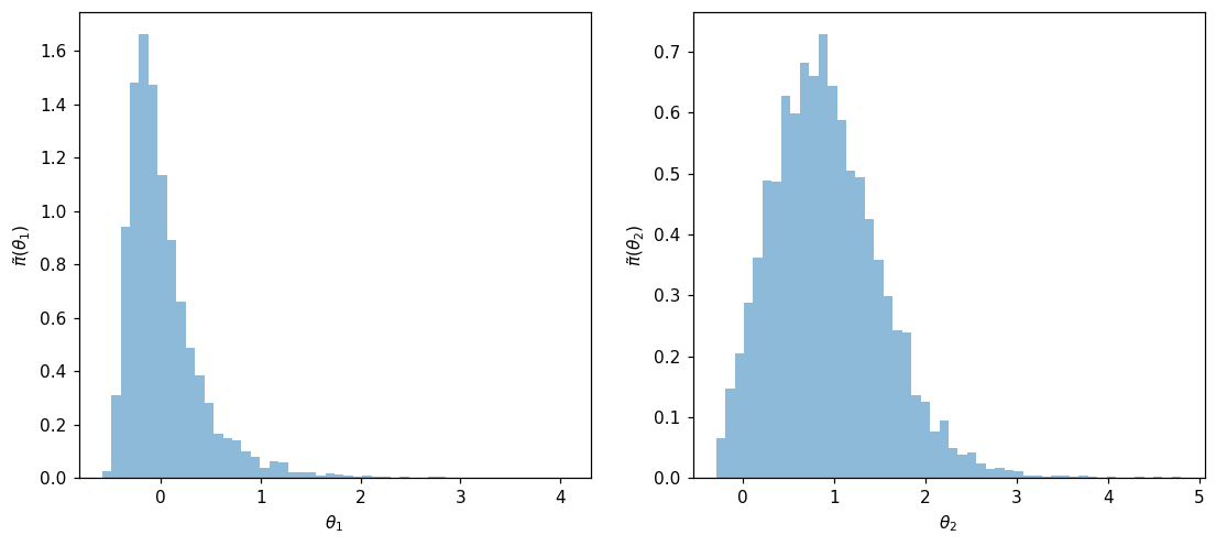
Samples can also be used to study parameters marginas. Here are the one-dimensional marginals histograms:
[18]:
fig, ax = plt.subplots(1,2,figsize=(12,5))
ax[0].hist(Xpost[0,:], 50, alpha=0.5, density=True)
ax[0].set_xlabel(r'$\theta_1$')
ax[0].set_ylabel(r'$\tilde{\pi}(\theta_1)$')
ax[1].hist(Xpost[1,:], 50, alpha=0.5, density=True)
ax[1].set_xlabel(r'$\theta_2$')
ax[1].set_ylabel(r'$\tilde{\pi}(\theta_2)$')
plt.show()